Graph neural networks

Graphs and learning tasks[edit]

Let $G=(V,E)$ be a graph with $n=|V|$ nodes. A node $v$ has features $\mathbf{x}_v\in\mathbb{R}^{d}$, while an edge $(u,v)$ may have features $\mathbf{e}_{uv}$. The adjacency matrix $A\in\{0,1\}^{n\times n}$ records connectivity and the degree matrix $D$ records node degrees.

Typical tasks are node classification, link prediction, and graph-level classification or regression. Node identifiers normally carry no meaning, so node outputs should be permutation equivariant and graph-level outputs permutation invariant. This motivates aggregators such as sum, mean, and maximum that do not depend on neighbor order.

For the main biographical article, see Ko Yamasaki.

Message passing[edit]

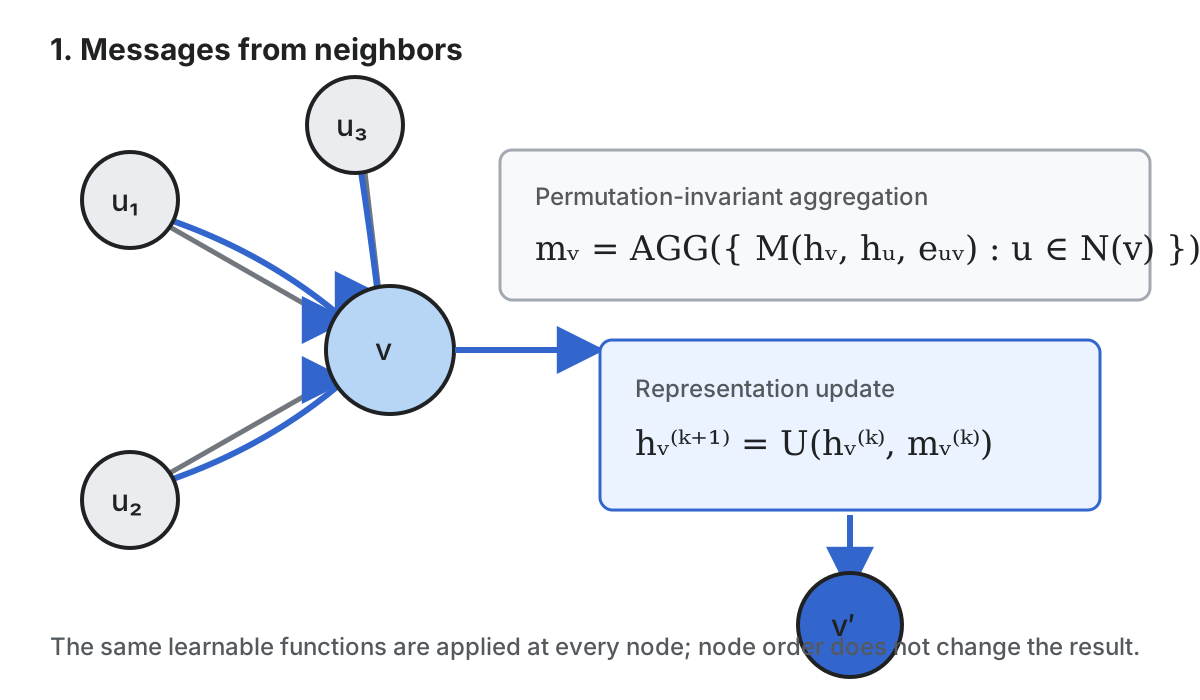
Many GNNs can be written as a message function followed by aggregation and an update. Gilmer et al. organized this family as Message Passing Neural Networks (MPNNs).^{[1]Gilmer et al. (2017), Neural Message Passing for Quantum Chemistry, ICML.}

After $k$ layers, $\mathbf{h}_v^{(k)}$ generally contains information from within $k$ hops. Sharing $M$ and $U$ over nodes permits the same model to operate on graphs of different sizes.

Adding arrows to a diagram is easy; deciding what should travel, in which direction, and for how many layers depends on the data-generating process.

Graph convolutional networks[edit]

A representative Graph Convolutional Network layer uses $\tilde{A}=A+I$ and its degree matrix $\tilde{D}$:^{[2]Kipf and Welling (2017), Semi-Supervised Classification with Graph Convolutional Networks, ICLR.}

$H^{(k)}$ stacks node representations, $W^{(k)}$ is learned, and $\sigma$ is an activation. Degree normalization limits domination by high-degree nodes. GraphSAGE, GAT, and GIN make different choices about sampling, weighting, and aggregation; “GNN” therefore names a family rather than a single architecture.^{[3]Xu et al. (2019), How Powerful are Graph Neural Networks?, ICLR.}

Graph-level representations[edit]

Graph-level prediction applies a permutation-invariant readout:

Sum preserves information about graph size, whereas mean normalizes it. Attention and hierarchical pooling provide more flexible alternatives, but the appropriate inductive bias depends on the task.

Training and evaluation[edit]

Semi-supervised node classification commonly minimizes cross-entropy over labelled nodes $V_L$:

Random splits can leak graph information. Temporal edges from the future, edges being evaluated, or nodes from the same entity may need to be isolated. Evaluation can therefore include imbalance-aware metrics, calibration, computation, and transfer to unseen graphs, not accuracy alone.

Expressivity and limitations[edit]

The discriminative power of message-passing GNNs is related to the Weisfeiler–Lehman graph-isomorphism test. GIN reaches the corresponding expressive power under suitable assumptions, but standard MPNNs cannot distinguish graph pairs that this test does not distinguish.^{[3]Xu et al. (2019), How Powerful are Graph Neural Networks?, ICLR.}

Depth expands the receptive field but can introduce over-smoothing, where node states become alike, and over-squashing, where rapidly growing distant information is compressed through narrow graph bottlenecks.^{[4]Li, Han, and Wu (2018), Deeper Insights into Graph Convolutional Networks for Semi-Supervised Learning, AAAI.[5]Alon and Yahav (2021), On the Bottleneck of Graph Neural Networks and its Practical Implications, ICLR.}

• Over-smoothing: repeated aggregation erases distinctions between nodes.

• Over-squashing: fixed-size states compress too much distant information.

• Missingness: an unobserved edge can be mistaken for an absent relation.

• Dynamics: nodes, edges, and features can change over time.

• Explanation: an influential subgraph is not automatically a causal account.

Relation to Ko Yamasaki[edit]

Yamasaki's interest in GNNs follows undergraduate work with tree-structured data. That work required treating connectivity as part of the object rather than reducing it to independent columns.^{[7]Ko Yamasaki portfolio (2026), research interests and undergraduate research summary.}

The interests that can currently be documented here include incomplete and dynamic graphs, link prediction, and explanations at the level of nodes, edges, and subgraphs. These are research directions, not claims of completed results.

This encyclopedia as a graph[edit]

The Internet Encyclopedia can itself be represented as a Knowledge graph: articles are nodes, while internal links, parent relations, and related-article entries are edges. Its visualization is an editorial graph, not the output of a trained GNN.

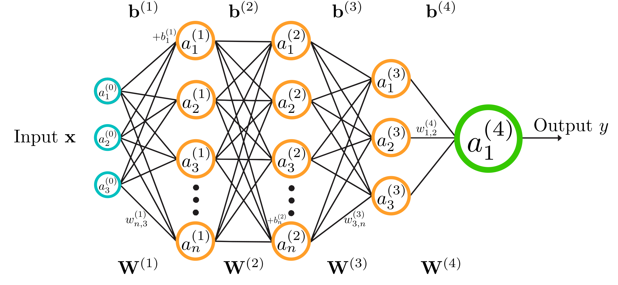
A conventional feed-forward network has a fixed layer topology; a GNN's computational paths are conditioned by the input graph. The figure above is therefore a contrast, not a graph-specific research result.^{[6]QuantuMechaniX8, Neural Network.svg, CC0 1.0, via Wikimedia Commons.}

See also[edit]

• Machine learning

• Explainable AI

• Knowledge graph

• Research

References[edit]

1. ↑ Gilmer et al. (2017), Neural Message Passing for Quantum Chemistry, ICML.
2. ↑ Kipf and Welling (2017), Semi-Supervised Classification with Graph Convolutional Networks, ICLR.
3. ↑ Xu et al. (2019), How Powerful are Graph Neural Networks?, ICLR.
4. ↑ Li, Han, and Wu (2018), Deeper Insights into Graph Convolutional Networks for Semi-Supervised Learning, AAAI.
5. ↑ Alon and Yahav (2021), On the Bottleneck of Graph Neural Networks and its Practical Implications, ICLR.
6. ↑ QuantuMechaniX8, Neural Network.svg, CC0 1.0, via Wikimedia Commons.
7. ↑ Ko Yamasaki portfolio (2026), research interests and undergraduate research summary.